Lab 1G: What’s the FREQ?

Lab 1G - What's the FREQ?

Directions: Follow along with the slides, completing the questions in blue on your computer, and answering the questions in red in your journal.

Clean it up!

In Lab 1F, we saw how we could clean data to make it easier to use and analyze.

– You cleaned a small set of variables from the American Time Use (ATU) survey.

– The process of cleaning and then analyzing data is very common in Data Science.
In this lab, we'll learn how we can create frequency tables to detect relationships between categorical variables.

– For the sake of consistency, rather than using the data that you cleaned, you will use the pre-loaded ATU data.

– Use the data() function to load the atu_clean data file to use in this lab.

How do we summarize categorical variables?

When we're dealing with categorical variables, we can't just calculate an average to describe a typical value.

– (Honestly, what's the average of categories orange, apple and banana, for instance?)
When trying to describe categorical variables with numbers, we calculate frequency tables

Frequency tables?

When it comes to categories, about all you can do is count or tally how often each category comes up in the data.
Fill in the blanks below to answer the following: How many more females than males are there in our ATU data?
```
tally(~ ____, data = ____)
```

2-way Frequency Tables

Counting the categories of a single variable is nice, but often times we want to make comparisons.
For example, what if we wanted to answer the question:

– Does one gender seem to have a higher occurrence of physical challenges than the other?
We could use the following plot to try and answer this question:
```
bargraph(~phys_challenge | gender, data = atu_clean)
```

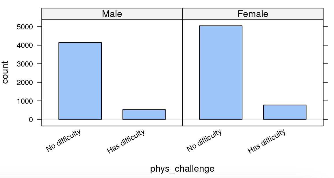
The split bargraph helps us get an idea of the answer to the question, but we need to provide precise values.
Use a line of code, that’s similar to how we facet plots, to obtain a tally of the number of people with physical challenges and their genders.
- Write down the resulting table.

Interpreting 2-way frequency tables

Recall that there were 1153 more women than men in our data set.

– If there are more women, then we might expect women to have more physical challenges (compared to men).
Instead of using counts we use percentages.
Include: format = "percent" as an option to the code you used to make your 2-way frequency table.

– Does one gender seem to have a higher occurrence of physical challenges than the other? If so, which one and explain your reasoning?
It’s often helpful to display totals in our 2-way frequency tables.

– To include them, include margins = TRUE as an option in the tally function.

Conditional Relative Frequencies

There is as difference between phys_challenge | gender and gender | phys_challenge!

tally(~phys_challenge | gender, data = atu_clean, margin = TRUE)

##                 gender
## phys_challenge   Male Female
##   No difficulty  4140   5048
##   Has difficulty  530    775
##   Total          4670   5823

tally(~gender | phys_challenge, data = atu_clean, margin = TRUE)

##         phys_challenge
## gender   No difficulty Has difficulty
##   Male            4140            530
##   Female          5048            775
##   Total           9188           1305

Conditional Relative Frequencies, continued

At first glance, the two-way frequency tables might look similar (especially when the margin option is excluded). Notice, however, that the totals are different.
The totals are telling us that R calculates conditional frequencies by column!
What does this mean?

– In the first two-way frequency table the groups being compared are Male and Female on the distribution of physical challenges.

– In the second two-way frequency table the groups being compared are the people with No difficulty and those that Has difficulty on the distribution of gender.
Add the option format = "percent" to the first tally function. How were the percents calculated? Interpret what they mean.

On your own

Describe what happens if you create a 2-way frequency table with a numerical variable and a categorical variable.
How are the types of statistical investigative questions that 2-way frequency tables can answer different than 1-way frequency tables?
Which gender has a higher rate of part time employment?