Lesson 3: Data Structures

Objective:

Students will learn that data can be represented in rectangular format.

Materials:

DS journals (must be available during every lesson)
Stick Figures cutouts (see lesson 2)

Vocabulary:

variables numerical variables categorical variables rows columns rectangular or spreadsheet format variability

Essential Concepts:

Variables record values that vary. By organizing data into rectangular format, we can easily see the characteristics of observations by reading across a row, or we can see the variability in a variable by reading down the column. Computers can easily process data when it is rectangular format.

Lesson:

Remind students that they briefly learned what variables are during the previous lesson. Have students create their own definitions of the term “variables” and share their responses with their teams. Select a few students in the class to share out their definitions and discuss what could be modified (if anything) to create a more complete definition.
Using the Stick Figure information from Lesson 2, allow the class to come up with a set of variable names that describe the different categories of information. Note that it is best when variable names are short (one to three words). The variable names for the Stick Figures data could possibly be:
1. Name
2. Height
3. GPA
4. Shoe or Shoe Type
5. Sport
6. Friends or Number of Friends
Next, have a class discussion about how the values from “Shoe” are different than the values from “Height.”
1. The values from “Shoe” are either “sneakers” or “sandals”.
  
  Note: Other terms for these shoes are acceptable – e.g., tennis shoes, flip flops, closed-toe, open-toe, etc.
2. The values from “Height” are 72, 68, 61, 66, 65, 61, 67, and 64.
Students should notice that the “Shoe” variable consists of categories or groupings, and the “Height” variable consists of numbers. Therefore, we can classify variables into two types: categorical variables and numerical variables. Typically, categorical variables represent values that have words, while numerical variables represent values that have numbers.

Note: Categorical variables can sometimes be coded as numbers (e.g., “Gender” could have values 0 and 1, where 0=Male and 1=Female).
As a class, determine which variables from the Stick Figures data are numerical, and which variables are categorical. The students should create two lists in their DS journals similar to the ones below (the correct classifications are in grey):

    Numerical     Categorical

1. Height           1. Name

2. GPA               2. Shoe

3. Friends         3. Sport
Explain that although we can understand many different representations of data (as evidenced by the posters from Lesson 2), computers are not as capable. Instead, we need to organize data in a structured way so that a computer can read and interpret them.
One way to organize the data is to create a data table that consists of rows and columns. We can define this type of organization as rectangular format, or spreadsheet format.
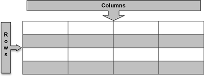
Display a generic table on the board (see example below) and explain that the columns are the vertical portions of the table, while the rows are the horizontal portions. Another way to think of it is that columns go from top to bottom, and rows go from left to right.
Ask students:
1. What should each row represent? Each row should represent one observation, or one stick figure person in this case.
2. What should each column represent? Each column should represent one variable. As you go down a column, all the values represent the same characteristic (e.g., Height).
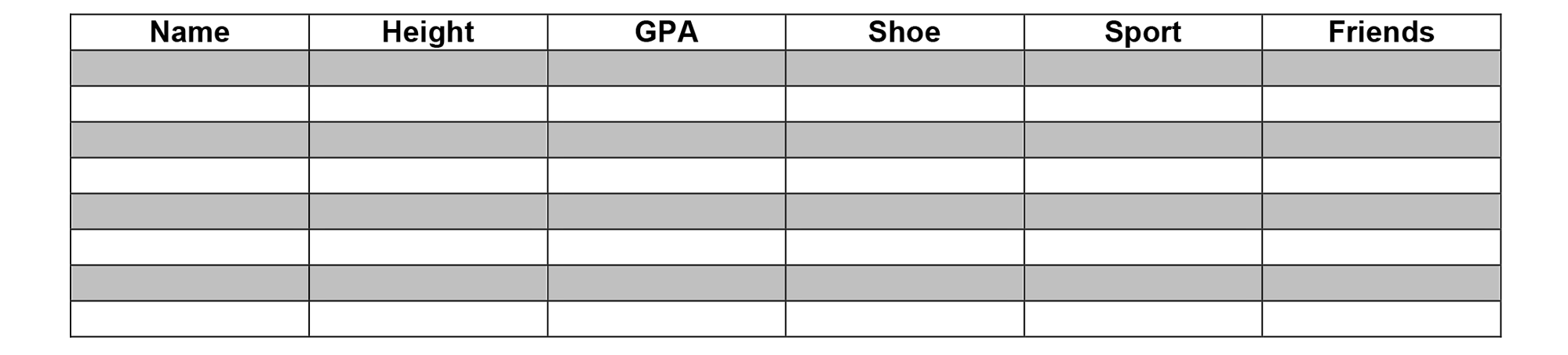
On the board, draw the following table and have the students copy it into their DS journals (be sure to use variable names agreed upon by the class):
In teams, students should complete the data table using all 8 of the Stick Figures cards. Each row of the table should represent one person on a card.
Engage the class in a discussion with the following questions:
1. Do any of the people in the data have the same value for a given variable? In other words, does a value appear more than once in a column? Give two examples. Answers will vary. One example could be that Dakota, Kamryn, Emerson, and London all wear sneakers. Another example could be that Charlie and Jessie are both 61 inches tall.
2. Do any of the people in the data have different values for a given variable? Absolutely. There are many instances of this in the data table.
Discuss the term variability. As in question (b) above, the values for each variable vary depending on which person we are observing. This shows that the data has variability, and the first step in any investigation is to notice variability. We can see the relationship between the terms variable and variability. The word “variable” indicates that values vary.

Class Scribes:

One team of students will give a brief talk to discuss what they think the 3 most important topics of the day were.