Lesson 13: The Horror Movie Shuffle

Objective:

Students will understand that, just by chance, we will see differences between two groups. They will understand that these differences are usually small. Specifically, they will learn that we can determine if outcomes are due to chance for categorical variables by calculating differences in the proportions between two groups.

Materials:

3” x 5” cards (1 per student)

Vocabulary:

chance simulations randomness shuffle

Essential Concepts:

We can "shuffle" data based on categorical variables. The statistic we use is the difference in proportions. The distribution we form by shuffling represents what happens if chance were the only factor at play. If the actual observed difference in proportions is near the center of this shuffling distribution, then we would conclude that chance is a good explanation for the difference. But if it is extreme (in the tails or off the charts), then we should conclude that chance is NOT to blame. Sometimes, the apparent difference between groups is caused by chance.

Lesson:

Data Collection Monitoring: Display the IDS Campaign Monitoring Tool, found at https://portal.idsucla.org. Click on Campaign Monitor and sign in.
Inform students that you will be monitoring their data collection. Ask:
1. Who has collected the most data so far? See User List and sort by Total.
2. How many active users are there? How many inactive users are there? Click on pie chart.
3. How many responses were submitted yesterday and today? See Total Responses.
4. How many responses have been shared? How many remain private? Click on pie chart.
5. Using TPS, ask students to think about what they can do to increase their data collection.
Conduct a discussion about the data that has been collected.
Have students recall what they have learned about chance (see Lesson 8). Synonyms: possibility, prospect, expectation, unintentional, unplanned. The actual definition of chance is “a possibility of something happening.”
To expand on the flow chart from Lesson 9 (chance → probability → simulations), explain that we can use simulations to show that sometimes, when we think two groups are different, the difference is really just because of chance, or randomness, and does not mean anything. This brings us back to “chance” in the flow chart.
Remind students that a simulation is a model for creating random outcomes. Randomness means that something just happens without a specific order.
In pairs, ask students to name situations where two groups could be compared, and then have the students record these situations in their DS journals. Some examples include:

• Men earn more money than women for some work.

• Basketball players are faster runners than baseball players.

• Los Angeles students are smarter than .

• UCLA football players are better athletes than USC football players.

• You and a friend flipped a coin 10 times, and you got more "heads."
Then, ask students to write next to each situation whether they think the differences are either real or due to chance because sometimes differences between two groups are real, but sometimes they might just be due to chance, and they will be learning ways to tell the difference.
Explain to the class that we are interested in finding out who will survive by the end of a horror movie. Ask the students:
1. Do you think men and women have an equal likelihood of surviving by the end of a horror movie? Answers will vary by class.
Have a few students share out their opinions along with their reasoning.
Inform the students that they will be pretending to be actors from horror movies during today’s lesson.
Explain that data from horror movies (sometimes called slasher films) were collected of 485 characters from 50 films. For each character, 2 variables were recorded: Gender and Survival. The values for Gender were “Male” and “Female.” The values for Survival were “Dies” and “Survives.”

Gender

Survival Female Male

Dies 172 228

Survives 50 35

Total 222 263

Notice that there were more male characters than female characters and that most characters in slasher films do not survive.
From this data, the proportion of survivors was calculated for each gender. In other words, for all female characters, the number of female survivors was divided by the total number of females. Similarly, for all male characters, the number of male survivors was divided by the total number of males.

$\frac{\#('' Female '' \&'' Survives '')}{\#('' Female '')}\ \ \ or\ \ \ \frac{\#('' Male '' \&'' Survives '')}{\#('' Male '')}$
The percent of females who survived by the end of a horror movie was about 23%, and the percent of males who survived by the end of a horror movie was about 13%. Ask the students:
1. Is this what you expected? (Refer back to the discussion from Step 9.) Answers will vary by class. If students thought males would survive more often, then these results would be unexpected. If students thought females would survive more often, then these results would be exactly what they expected. If students thought there was an equal likelihood of survival, these results would also be surprising.
2. What is the difference in the proportions of survival rates between genders? What does this mean in the context of surviving a horror movie? The difference is 23% - 13% = 10%. This means that 10% more women characters survived than men.
3. Is this difference “big” or “small”? How can they define what is “big” and what is “small?” Answers will vary by class. Upon first glance, it may seem like 10% is a big difference, but we do not know for sure.
Explain that they will participate in an activity to determine if the 10% difference seen in the actual data set is big or small. This will help them determine if there really is a difference in survival rates for males versus females, or if the 10% difference was just due to chance.
Split the class into two groups, 46% of them on one side of the room and the other 54% on the other side of the room. Tell the smaller group they have been assigned to play female characters in the horror movie (regardless of their gender) and tell the larger group that they have been assigned to play male characters in the horror movie (regardless of their gender). Once those groups have been created, have the class calculate the number of students in each group that would have survived a horror film using the actual proportions given in Step 14.

For example: For a class of 30 students:

• 46% of 30 (0.46x30) ≈ 14 students representing female characters.

• Of those 14 female characters, 23%, or 3 (0.23x14 ≈ 3), are survivors.

• The remaining 16 students (30 – 14 = 16) represent male characters.

• Of those 16 male characters, 13%, or 2 (0.13x16 ≈ 2), are survivors.
Each group should then decide which students will be survivors. Using the 3” x 5” cards, students should write either “dies” or “survives” on their card.

For example (continued from above):

Three of the female characters are survivors; so 3 female characters from the group should write “survives” on their cards. The rest of the group should write “dies” on their cards.

Two of the male characters are survivors; so 2 male characters from the group should write “survives” on their cards. The rest of the group should write “dies" on their cards.
Explain to students that IF there really is no difference between genders in horror films, then the characters who survived would only have done so by chance. In other words, males and females would have an equal likelihood of surviving. Have students discuss the following questions:
1. How many total people in our class are survivors? What is the total proportion of survivors? Answers will vary by class. Using the example above, there would be a total of 5 survivors from the class of 30 students. The proportion of survivors would be 5/30 = 0.17 = 17%
2. How many of the survivors would we expect to be male? How many would we expect to be female? Answers will vary by class. Using the example above, we would expect to see 17% of males and 17% of females survive since that was the overall proportion of survivors. So, we would expect 0.17x16 ≈ 3 male survivors, and 0.17x14 ≈ 2 female survivors.
Collect all of the 3” x 5” cards from the students and explain that you are going to shuffle the cards and redistribute them so that their genders have no influence on whether or not they survive the horror movie.
Visibly shuffle the survives/dies cards to create a random shuffle. Once the cards have been well-shuffled, pass them back out to the students face down. After all the cards are given out, each group should identify the number of people that are survivors and calculate the corresponding proportion of the survivors.

On the board, create a table to display the proportions of survivors for each gender, and include a column for the difference (female survivors – male survivors). Fill in the table with the values the students found in Step 20. Note: The first row has been filled in with the example data from above BEFORE the shuffles have taken place. Exact numbers were not used so that the proportions would match the actual horror movie data set.

# of Female Survivors	# of Male Survivors	Proportion of Female Survivors	Proportion of Male Survivors	Difference in Proportions (Female – Male)
3.22	2.08	3.22/14 = 0.23	2.08/16 = 0.13	0.23 – 0.13 = 0.10
?

Note that values in the “Difference in Proportions” column can be positive or negative because sometimes more women will survive, and other times more men will survive.
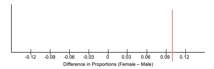
Draw a dotplot on the board labeled “Difference in Proportions.” Include a vertical line at 10% to represent the actual difference in gender survival rates in real horror movies (see example below).
Using the information from Steps 20 and 21, place a dot at the corresponding value for the shuffled data’s difference in proportions. Ask the students:
1. How does this difference compare to the actual data set’s difference of 10%? Answers will vary by class. Most likely, the difference in proportions will be much smaller than 10%. In fact, the difference in proportions will be centered around 0.
Repeat Steps 19 – 24 a few more times (depending on how much class time you have available).
Ask the students to record their responses to the following questions:
1. What was the biggest difference we saw from our shuffles? What was the smallest? Answers will vary by class.
2. What do you think this dotplot would look like if we shuffled our survival cards 1000 times? The dotplot would look roughly symmetric and centered around 0, meaning that if there were no relationship between a character’s gender and whether or not they survive, the difference in proportions would typically be 0.
Have a discussion about how the actual difference in gender survival (10%) is rarely seen when we assign “survives” or “dies” just by chance (aka when shuffling). What does this mean in terms of who will die in actual horror movies? Since we never (or rarely) saw a 10% difference in the proportions of female survivors versus male survivors, it seems that horror movies actually favor female survivors.
Ask the students:
1. If you were going to be cast in a horror movie, would you want to be a male character or a female character? You would want to be a female character because they are more likely to survive by the end of the film.
Inform the students that they will learn how to shuffle in RStudio in order to determine if an event is real or simply due to chance.

Class Scribes:

One team of students will give a brief talk to discuss what they think the 3 most important topics of the day were.

Homework & Next Day

For the next 5 days, students will collect data for the Stress/Chill campaign either through the UCLA IDS UCLA App or via web browser at https://portal.idsucla.org

LAB 2E: The Horror Movie Shuffle

Complete Lab 2E prior to Lesson 14.

	Gender
Survival	Female	Male
Dies	172	228
Survives	50	35
Total	222	263