LAB 4C: Cross-Validation
Lab 4C - Cross-Validation
Directions: Follow along with the slides, completing the questions in blue on your computer, and answering the questions in red in your journal.
What is cross-validation?
-
In the previous two labs, we learned how to:
– Create a linear model predicting
heightfrom thearm_spandata (4A).– See how well our model predicts
heighton thearm_spandata by computing mean squared error (MSE)(4B). -
In this lab, we will see how well our model predicts the heights of people we haven't yet measured.
-
To do this, we will use a method called cross-validation.
-
Cross-validation consists of three steps:
– Step 1: Split the data into training and test sets.
– Step 2: Create a model using the training set.
– Step 3: Use this model to make predictions on the test set.
Step 1: train-test split
-
Waiting for new observations can take a long time. The U.S. takes a census of its population once every 10 years, for example.
-
Instead of waiting for new observations, data scientists will take their current data and divide it into two distinct sets.
-
Split the
arm_spandata intotrainingandtestsets using the following two steps. -
First, fill in the blanks below to randomly select which rows of
arm_spanwill go into thetrainingset.set.seed(123) train_rows <- sample(1:____, size = 85) -
Second, use the
slicefunction to create two dataframes: one calledtrainconsisting of thetrain_rows, and another calledtestconsisting of the remaining rows ofarm_span.train <- slice(arm_span, ____) test <- slice(____, - ____) -
Explain these lines of code and describe the
trainandtestdatasets.
Aside: set.seed()
-
When we split data, we're randomly separating our observations into training and testing sets.
– It's important to notice that no single observation will be placed in both sets.
-
Because we're splitting the data sets randomly, our models can also vary slightly, person-to-person.
– This is why it's important to use
set.seed. -
By using
set.seed, we're able to reproduce the random splitting so that each person's model outputs the same results.Whenever you split data into training and testing, always use
set.seedfirst.
Aside: train-test ratio
-
When splitting data into training and testing sets, we need to have enough observations in our data so that we can build a good model.
– This is why we kept 85 observations in our
trainingdata. -
As datasets grow larger, we can use a larger proportion of the data to
testwith.
Step 2: train the model
-
Step 2 is to create a linear model relating
heightandarmspanusing thetrainingdata. -
Fit a line of best fit model to our
trainingdata and assign it the namebest_train. -
Recall that the slope and intercept of our linear model are chosen to minimize MSE.
-
Since the MSE being minimized is from the training data, we can call it training MSE.
Step 3: test the model
-
Step 3 is to use the model we built on the
trainingdata to make predictions on thetestdata. -
Note that we are NOT recomputing the slope and intercept to fit the test data best. We use the same slope and intercept that were computed in step 2.
-
Because we're using the line of best fit, we can use the
predict()function we introduced in the last lab to make predictions.– Fill in the blanks below to add predicted heights to our
testdata:test <- mutate(test, ____ = predict(best_train, newdata = ____)) -
Hint: the
predictfunction without the argumentnewdatawill output predictions on thetrainingdata. To output predictions on thetestdata, supply thetestdata to thenewdataargument. -
Calculate the test MSE in the same way as you did in the previous lab (test MSE is simply MSE of the predictions on the test data).
Recap
-
Another way to describe the three steps is
-
Step 1: Split the data into
trainingandtestsets. -
Step 2: Choose a slope and intercept that minimize training MSE.
-
Step 3: Using the same slope and intercept from step 2, make predictions on the
testset, and use these predictions to compute test MSE.
-
-
This begs the question, why do we care about test MSE?
Why cross-validate?
-
Why go to all this trouble to compute test MSE when we could just compute MSE on the original dataset?
-
When we compute MSE on the original dataset, we are measuring the ability of a model to make predictions on the current batch of data.
-
Relying on a single dataset can lead to models that are so specific to the current batch of data that they're unable to make good predictions for future observations.
– This phenomenon is known as overfitting.
-
By splitting the data into a training and test set, we are hiding a proportion of the data from the model. This emulates future observations, which are unseen.
-
Test MSE estimates the ability of a model to make predictions of future observations.
Example of overfitting
-
The following example motivates cross-validation by illustrating the dangers of overfitting.
-
We randomly select 7 points from the
arm_spandataset and fit two models: a linear model, and a polynomial model.– You will learn how to fit a polynomial model in the next lab.
-
Below is a plot of these 7
trainingpoints, and two curves representing the value of height each model would predict given a value of armspan.
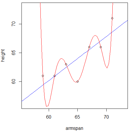
-
Which model does a better job of predicting the 7
trainingpoints? -
Which model do you think will do a better job of predicting the rest of the data?
Example of overfitting, continued
- Below is a plot of the rest of the
arm_spandataset, along with the predictions each model would make.
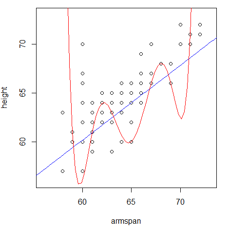
- Which model does a better job of generalizing to the rest of the
arm_spandataset?