Lesson 10: What’s the Best Line?
Lesson 10: What's the Best Line?
Objective:
Students will understand that the mean squared error (MSE) is a way to assess the fit of a linear model. The MSE measures the total squared distances between all the data values from the line of best fit and divides it by the number of observations in the dataset.
Materials:
-
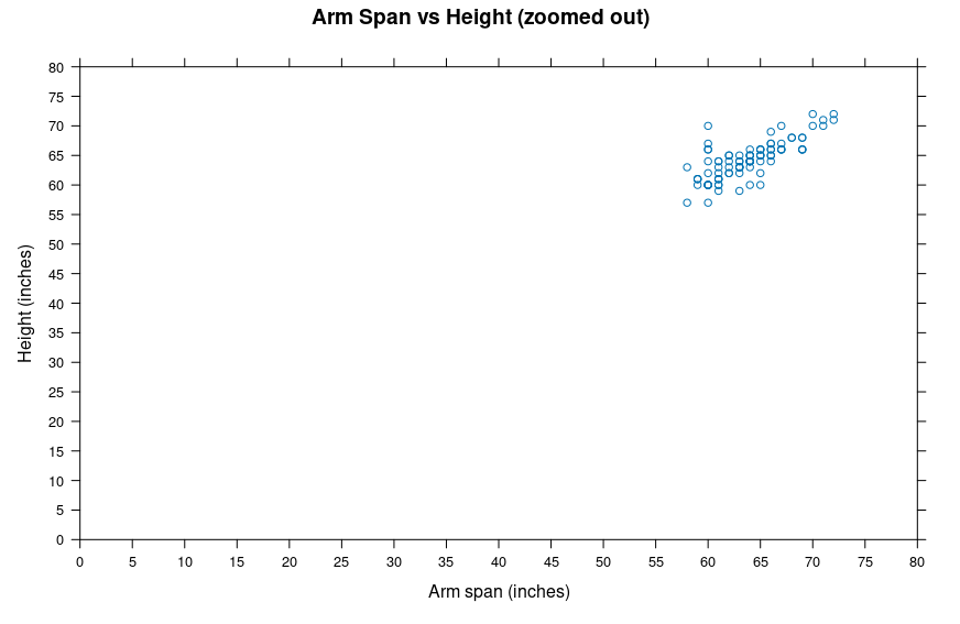
Arm Span vs. Height Scatterplot (LMR_4.9_Arm Span vs Height) from lesson 8
-
Testing Line of Best Fit handout (LMR_4.11_Testing Line of Best Fit)
Vocabulary:
regression line observed value predicted value
Essential Concepts:
Essential Concepts:
The regression line can be used to make good predictions about values of y for any given value of x. This works for exactly the same reason the mean works well for one variable: the predictions will make your score on the mean squared errors as small as possible.
Lesson:
-
Ask student teams to refer back to the Arm Span vs. Height handout (LMR_4.9) but this time have them look at the zoomed out scatterplot.
-
Using their understanding of a line of best fit from The Spaghetti Line lesson and Lab 4A, have them draw (or use strands of spaghetti) what they believe to be the line of best fit for the data.
Note: They can use their equations from Lab 4A as a guide but note that it will be difficult to plot decimals on this scatterplot. -
Ask students: How does this line compare to the lines from the team posters in The Spaghetti Line lesson? Answers will vary but students may notice that the y-intercepts may be similar or that the overall slope appears similar (they are not writing an equation for the line in step 2, but they may notice where their line intercepts the y-axis and/or the steepness of the line, i.e., slope).
-
Reveal the equation of the line of best fit for the Arm Span vs. Height data and ask students to check their equations from Lab 4A:
Note: Any time a hat is on top of a variable, this means we are making “predicted values” of that variable.
-
Whose equation came closest to the equation of the regression line? Ask the student whose equation came closest to share how he/she came up with the equation.
-
Inform students that the equation of the line is a rule that predicts the height based on a second variable, in this case, arm span. Data points are observed values and points on the line are predicted values.
-
Team discussion question:
Using the equation of the line of best fit provided, how can we predict the height of a student whose arm span is 67 inches?
-
What was the actual height for someone with an arm span of 67 inches? Answer: There are three points on our Arm Span vs Height scatterplot at an arm span of 67 inches; 66-inch height, 67-inch height, and 70-inch height.
-
How close was our predicted height? Answer: Our line of best fit predicted that someone with an arm span of 67 inches has a height of 66.5933 inches, which rounded to the nearest whole number is 67 inches. This is pretty close as it matches one of the possible heights for someone with an arm span of 67 inches in our data.
-
-
Remind students know that lines of best fit are also known as regression lines and they are models that can be used to make predictions.
-
Inform students that data scientists have a way of finding the best line. They choose the line so that the mean squared distances between the points and the line is as small as possible. Discuss with students:
-
What methods have we used so far? Answer: We've used Mean Squared Error and Mean Absolute Error (Lesson 7)
-
When is it appropriate to use each method? Answer: It was best to use Mean Squared Error when we were looking at mean and Mean Absolute Error when we were looking at median.
-
-
Distribute the Testing Line of Best Fit handout (LMR_4.11). Students will calculate MSE by using the distances between the actual heights (the points) and their predicted heights (the points on the line) of two different lines. They do this so that they can understand what those distances mean - that together they form our "error" that help us determine the best fitting line.
-
Discuss with students:
-
What did you have to do to your MSE value to make it useable for interpretation? Answer: We had to take the square root of our MSE value in order to convert it back to inches.
-
Which linear model was the better fit? How do you know? Answers will vary but this is where students should compare the MSE values - a smaller MSE indicates a smaller error, and therefore a better fit.
Note: Students may ask for an easier and/or faster way to calculate MSE. They will be using RStudio to calculate MSE in the next lab.
-
Class Scribes:
One team of students will give a brief talk to discuss what they think the 3 most important topics of the day were.
Homework & Next Day