Lesson 14: More Variables to Make Better Predictions
Lesson 14: More Variables to Make Better Predictions
Objective:
Students will see that different variables can be used to make predictions about the same outcome (response variable) and consider whether combining these variables could improve prediction accuracy.
Materials:
-
Advertising Plots Part 1 handout (LMR_4.17_Advertising Plots 1)
-
Advertising Plots Part 2 handout (LMR_4.18_Advertising Plots 2)
-
Article: How Long Can a Spinoff Like ‘Better Call Saul’ Last?
http://fivethirtyeight.com/features/how-long-can-a-spinoff-like-better-call-saul-last/
Vocabulary:
Essential Concepts:
Essential Concepts:
We can use scatterplots to assess which variables might lead to strong predictive models. Sometimes using several predictors in one model can produce stronger models.
Lesson:
-
Remind students that models are used to make predictions. Ask a volunteer to think of a TV show that had a “spinoff” and to name both of the shows. Ask if he/she knows whether or not the original was more or less successful than the spinoff. Then, ask the class: Is there a way to predict spinoff success?
-
Next, using the Talking to the Text instructional strategy, ask students to read the article titled: How Long Can a Spinoff Like Better Call Saul Last?
Note: If this is the first time using this strategy with your students, make sure you model/explain it before they begin reading it. See Instructional Strategies in Teacher Resources for a description.
-
After reading the article, ask students to discuss three Talking to the Text responses with a partner. You may set a time limit for each student to share with his/her partner.
-
Then, in teams, students will answer the following questions pertaining to the article:
-
What is the article trying to predict? Answer: The success of a spinoff show.
-
How many variables are used? Answer: Four - the original show name, the number of episodes of the original show, the name of the spinoff show, and the number of episodes of the spinoff show.
-
What other variables might affect a spinoff? Possible answers are budget or actors.
-
The dotted line in the plot is not a regression line. How would you draw a regression line to make predictions? Answers will vary but we would want to try to "fit" a line to the plotted data.
-
What other information would you like to know to predict a spinoff’s success? Answers will vary but may be similar to (c) above.
-
-
Allow students time to discuss and record their answers. Then conduct a share out of their responses to the discussion questions.
-
Discuss the following questions with the class:
-
What effect does advertising have on retail sales?
-
Where do stores advertise (What mediums do they use)? Does each method of advertisement reach the same people?
-
Does each method of advertisement have a similar effect? Or are some methods more effective than others?
-
-
Distribute the 3 plots from the Advertising Plots Part 1 handout (LMR_4.17) and inform the students about the data using the details below:
 (Plots are presented separately in the LMR)
-
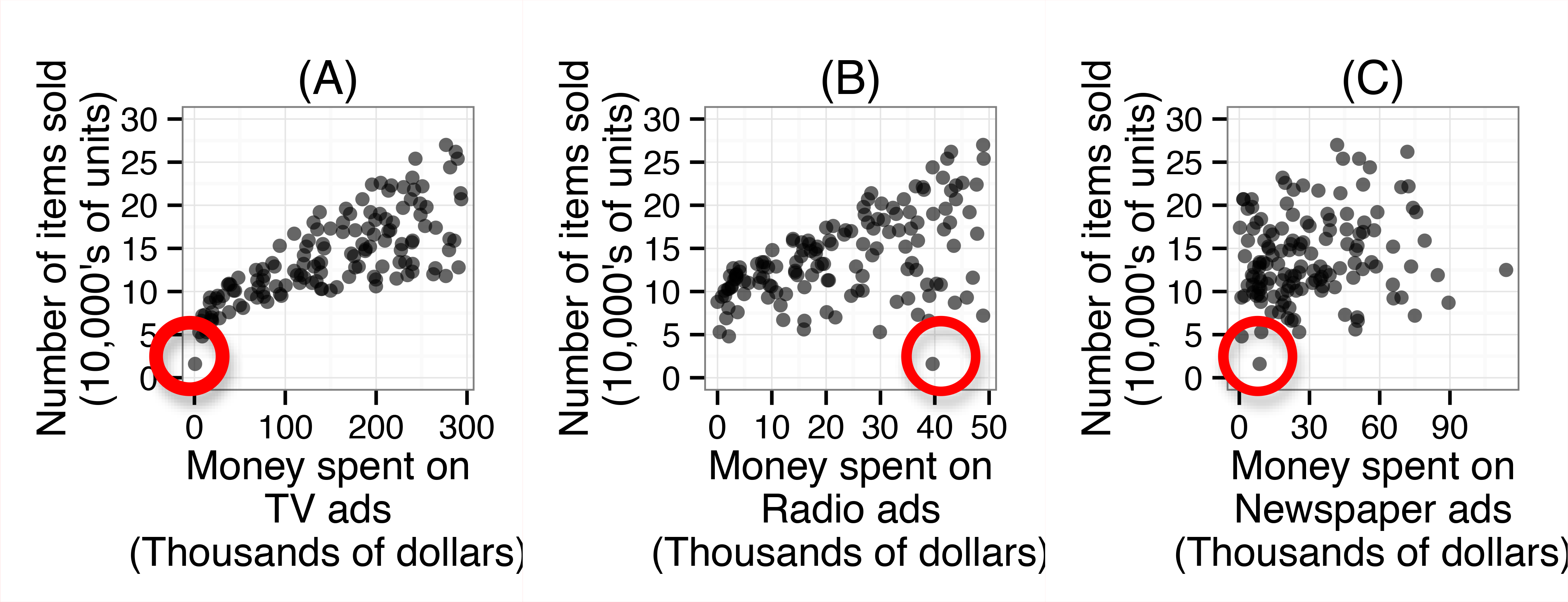
These 3 plots show the number of items sold by a retailer (in 200 different markets) and the amount of money the company spent on TV, Radio and Newspaper advertisements.
-
The data has 200 observations, one for each different market. A market is simply a location where an item is sold. For example, Los Angeles and San Francisco are two different markets.
-
Each observation has 4 variables: (1) The number of items sold (in 10’s of thousands of units), (2) the money spent on TV ads (in thousands of dollars), (3) the money spent on radio ads (in thousands of dollars), and (4) the money spent on newspaper ads (in thousands of dollars).
-
The data were collected using an observational study.
-
-
To illustrate a-d above, ask students to refer to plot A (TV ads) and circle the market in which this retailer sold the least number of items (see circles in plots above). Ask: How many items did this market sell? Answer: About 20,000 items. The actual number of items sold was 1.6 (in 10,000’s of units) which is 16,000 items. How much money did this retailer spend on TV ads in this market? Answer: This retailer spent zero dollars on TV ads. The actual amount the retailer spent on TV ads was 0.7 thousands of dollars, which is $700.
-
Students should then refer to plot B (Radio ads), find the same market (the one in which the retailer sold about 20,000 items) and circle it. Ask: How much money did the retailer spend on Radio ads in the same market? Answer: About 40 thousand dollars. The actual amount spent on Radio ads was 39.6 thousands of dollars, which is $39,600.
-
Finally, ask students to refer to plot C (Newspaper ads), find the same market (the one in which the retailer sold about 20,000 items), and circle it. Ask: How much money did the retailer spend on Newspaper ads in the same market? Answer: About 10 thousand dollars. About The actual amount spent on Newspaper ads is 8.7 thousands of dollars, which is $8,700

-
Based on the above plots, use a Pair-Share to discuss the following:
-
Describe the relationship between advertisements and the number of items sold. Answers will vary but we would expect the number of items sold to increase with increased advertisements.
-
Which type of advertisement is the most strongly correlated with the number of units sold? How can you tell? Answer: Plot A, TV advertisements, appears to be the most strongly correlated with the number of units sold. We can tell because the points are more closely packed/together than in plots B or C.
-
-
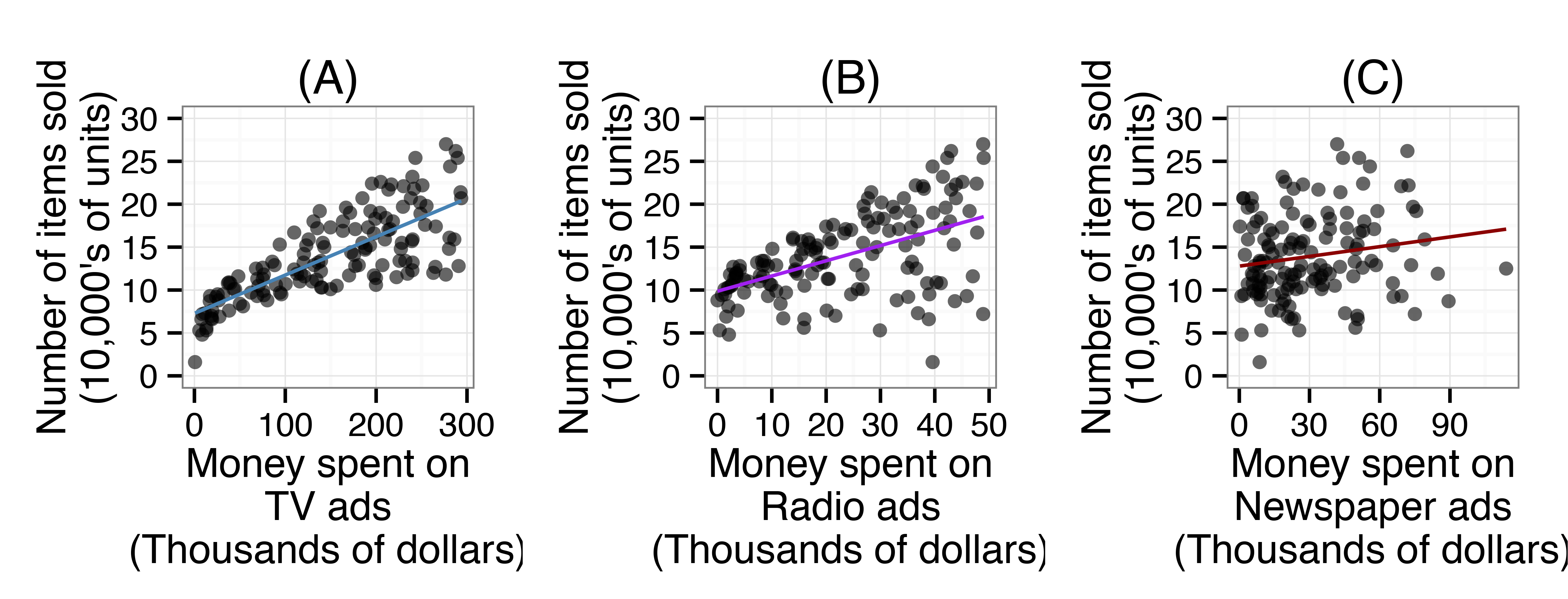
Distribute the Advertising Plots Part 2 handout (LMR_4.18), which contains plots A-C, but now include the line of best fit.
 (Plots are presented separately in the LMR)
 -
Ask students to recall from Lesson 7 that a method statisticians use to figure out which predicted values is closest to the actual data is the mean squared error (MSE).
-
In teams, ask students to discuss the following:
- How would you determine which plot would make the most accurate predictions? Answers will vary, but you would expect to hear something like: “the prediction line that has the least amount of distance to all the points on the plot would make the most accurate prediction because the predicted values will be closer to the actual data”.
-
Next, have students select a statement they think is best (a or b), then write a justification for their selection based on what they learned in this lesson. This may be completed as homework.
-
Combining multiple variables (e.g., TV and Newspaper ads, TV and Radio ads, TV, Radio, and Newspaper ads, etc.) into one model will lead to worse predictions because the variables that make poor predictions will contaminate those that make good predictions.
-
Combining multiple variables (e.g., TV and Newspaper ads, TV and Radio ads, TV, Radio, and Newspaper ads, etc.) into one model will lead to better predictions because the model can use more information to make predictions.
-
-
Inform students that RStudio has the capability of creating models that combine multiple variables to make predictions about another variable. For example, it can make a model to predict number of items sold using both money spent on TV and money spent on Newspaper ads. Students will learn more about it during the next lesson.
Class Scribes:
One team of students will give a brief talk to discuss what they think the 3 most important topics of the day were.
Homework
Students may continue writing their justifications for the selected statement in item 15 if they were unable to finish.